Tutorial: Binary Intrinsic Dimension
BID summary:
For non interacting random bit streams of length \(N\) it is possible to write the exact probability of observing Hamming distance $r = |:nbsphinx-math:boldsymbol{sigma}-\boldsymbol{\sigma}’|_H %=:nbsphinx-math:frac{N-boldsymbol{sigma} cdot boldsymbol{sigma}}{2} $ between two i.i.d samples \(\boldsymbol{\sigma}\) and \(\boldsymbol{\sigma}'\) as
\begin{equation} P_0(r) = \frac{1}{2^N} \binom{N}{r}. \tag{1} \end{equation}
For interacting spins, our model generalizes the previous expression to
\begin{equation} P(r)=C\frac{1}{2^{d(r)}}\binom{d(r)}{r}, \tag{2} \end{equation} where \(C\) is the normalization constant. Eq. 2 reduces to 1 for $ d(r) = N$ and \(C=1\). We empirically found that model 2 fits accurately the observed distributions, at least for small distances, if one retains the first two terms of the Taylor expansion: :nbsphinx-math:`begin{equation}
d(r)=d_0+d_1 , r tag{3}
end{equation}` where \(d_0\) and \(d_1\) are variational parameters. In order to infer them we minimize the Kullbac-Leibler divergence between the empirical probability of Hamming distances \(P_{emp}(r)\) and the model \(P(r)\) given by Eqs. 2 and 3,
- :nbsphinx-math:`begin{equation}
D_{KL}(P_{emp}||P) = sum_{r leq r_{max}} P_{emp}(r) log{frac{P_{emp}(r)}{P(r)}}, tag{4}
end{equation}` where \(r_{max}\) is a meta-parameter that allows constraining the fit to small distance if necessary ( i.e., we discard distances \(r>r_{max}\) from \(P_{emp}\), we show an example below). We fix \(r_{max}\) by taking it as the quantile of order \(\alpha_{max}\) of \(P_{emp}\), meaning
\begin{equation} \alpha_{max} = \sum_{r=0}^{r_{max}} P_{emp}(r), \tag{5} \end{equation} where \(\alpha_{max} \in [0,1]\). Ideally nothing depends qualitatively on \(\alpha_{max}\).
NOTE:
In the paper we call \(\alpha^* \equiv \alpha_{max}\) and \(r^* \equiv r_{max}\).
In practice we also define \(\alpha_{min}\) and \(r_{min}\) by
\begin{equation} \alpha_{min} = \sum_{r=0}^{r_{min}} P_{emp}(r), \tag{6} \end{equation} which allow to remove small distances (those with \(r<r_{min}\)) from \(P_{emp}\). These distances sometimes bring problems to the minimization of (4), for example when the histogram is poorly sampled in that regime.
Measuring the BID of random bits:
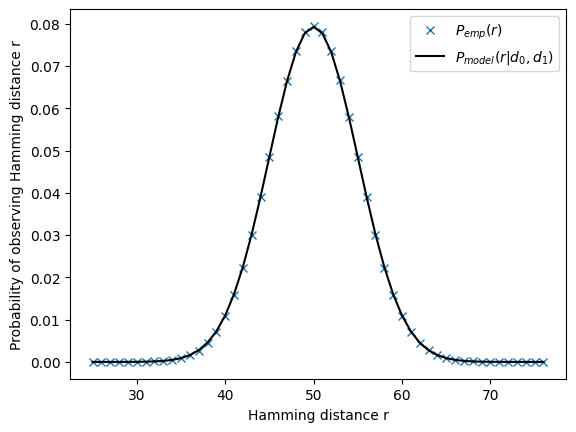
For \(N\) random spins the BID coincides with the number of variables. The solution for \(P(r)\) is exactly Eq. (1) and thus the optimization of (4) must give \(d_0=N\) and \(d_1=0\).
[1]:
import os
import numpy as np
import matplotlib.pyplot as plt

# this environmental variable must be set <before> the BID imports, to work with JAX double-precision
os.environ["JAX_ENABLE_X64"] = "True"
from dadapy.hamming import BID, Hamming

# REPRODUCIBILITY
seed = 1
np.random.seed(seed=seed)
[2]:
# RANDOM DATA
L = 100  # number of bits
Ns = 5000  # number of samples

# FORMAT NOTE: spins must be normalized to +-1
X = (2 * np.random.randint(low=0, high=2, size=(Ns, L)) - 1) # X.shape=(Ns,L)
[3]:
# DEFINING COORDINATES
H = Hamming(coordinates=X)

# COMPUTING DISTANCES
H.compute_distances() # stores the matrix of distances between samples in H.distances of shape (Ns,Ns)

# COMPUTING AND SAVING HISTOGRAM OF DISTANCES
histfolder = f'datasets/hamming/random_spins/L{L}/hist/'
filename = f'counts.txt'
H.D_histogram(compute_flag=1,            # if 0 the histograms are loaded instead of computed
              save=True,                 # we compute the histograms once and save time in the future
              resultsfolder=histfolder,  # folder where the histograms are saved
              filename=filename,
              )

# "H.D_histograms" defines the following attributes
idx = 5
print(f'{H.D_values[:idx]=}')  # vector containing the sampled distances
print(f'{H.D_counts[:idx]=}')  # vector containing how many times each distance was sampled
print(f'{H.D_probs[:idx]=}')   # same as "D_counts" but normalized by the total number of counts observed
H.D_values[:idx]=array([25, 26, 27, 28, 29], dtype=int32)
H.D_counts[:idx]=array([  4,   6,  34,  52, 120])
H.D_probs[:idx]=array([3.20e-07, 4.80e-07, 2.72e-06, 4.16e-06, 9.60e-06])
OPTIMIZATION
(See paper supp. inf for short description about the stochastic optimization performed)
[4]:
# PARAMETER DEFINITIONS FOR OPTIMIZATION
alphamin = 0        # order of min_quantile, to remove poorly sampled parts of the histogram if necessary (see Supp. Inf. of paper)
alphamax = 1        # order of max_quantile, to define r* (named rmax in the code).
delta = 5e-3        # stochastic optimization step size
Nsteps = int(1e5)   # number of optimization steps
export_results = 1  # flag to export d0,d1,logKL,Pemp,Pmodel after optimization (default=1)
export_logKLs = 1   # flag to export the logKLs during optimization (default=0)
optfolder0 = f"datasets/hamming/random_spins/L{L}/opt/"  # folder where optimization results are saved

B = BID(
    H=H,
    alphamin=alphamin,
    alphamax=alphamax,
    seed=seed,
    delta=delta,
    Nsteps=Nsteps,
    export_results=export_results,
    export_logKLs=export_logKLs,
    optfolder0=optfolder0,
    L=L,
)

B.computeBID()  # results are defined as attributes of B. They are also exported if export_results=1 (default)

print('')
print(f'{B.d0=}')
print(f'{B.d1=}')
print(f'{B.logKL=}')
print(f'{B.rmax=}')

# Note that B.intrinsic_dim is another alias for B.d0
print(f'\n {B.intrinsic_dim=}')
starting optimization
optimization took 0.0 minutes
d_0=99.574,d_1=0.008,logKL=-10.85

B.d0=99.57444692619558
B.d1=0.008277386221249374
B.logKL=-10.85470780641487
B.rmax=76

 B.intrinsic_dim=99.57444692619558
explicit model validation:
[47]:
fig,ax = plt.subplots(1)

# empirical distribution of distances
ax.plot(B.remp,
        B.Pemp,
        'x',
        label=r'$P_{emp}(r)$',
        )
# model fit
ax.plot(B.remp,
        B.Pmodel,
        '-',
        color='black',
        label=r'$P_{model}(r|d_0,d_1)$',
        )
plt.ylabel('Probability of observing Hamming distance r')
plt.xlabel('Hamming distance r')
plt.legend()
plt.show()
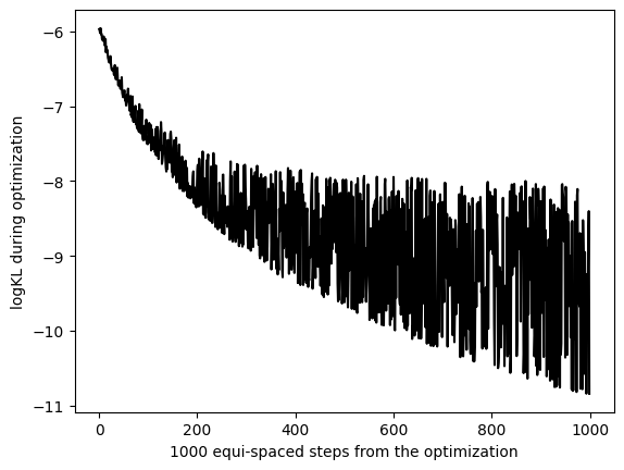
KL during optimization
Note that only random moves that minimize (4) are taken, and the rest are discarded. The following plot shows a subsampling of the proposed moves made by the optimizer.
[50]:
logKLs_opt = B.Op.logKLs # also importable by logKLs_opt = B.load_logKLs_opt()
figKL,axKL = plt.subplots()
axKL.plot(logKLs_opt,
          color='black',
          )
plt.ylabel('logKL during optimization')
plt.xlabel('1000 equi-spaced steps from the optimization')
plt.show()
2D Ising model
For this model we showed in our paper
The scaling of the BID with the number of spins
The temperature dependence of the BID
The fits of the model (2) to the empirical probabilities of distances for different temperatures
Below we show the full distribution of distances of this model, and what happens to the BID estimation when varying the meta paramater \(r_{max}\) defined in (4).
Some bibliography about the Ising model:
https://en.wikipedia.org/wiki/Ising_model
https://www.damtp.cam.ac.uk/user/tong/sft/one.pdf
Remember: the exact analytical temperature in the thermodynamic limit (infinite size limit) is \(T_c\approx 2.269\).
[31]:
import os
import numpy as np
import matplotlib.pyplot as plt

# this environmental variable must be set <before> the BID imports, to work with JAX double-precision
os.environ["JAX_ENABLE_X64"] = "True"
from dadapy.hamming import BID, Hamming
eps = 1E-7
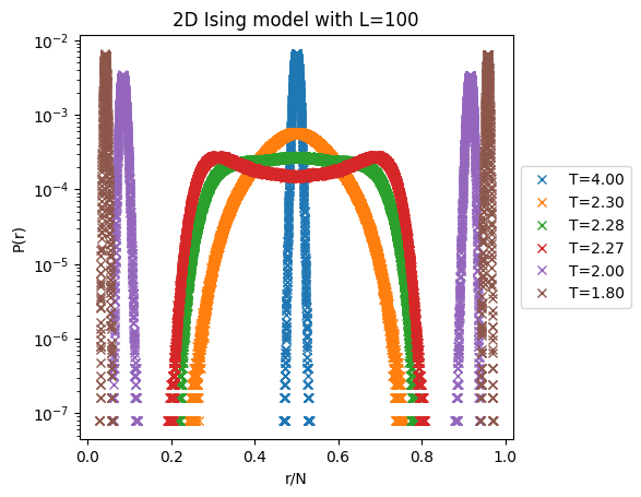
Histograms of distances show the phase transition:
We can see the phase transition in the histogram of all to all (Hamming-)distances, that becomes bimodal due to the presence of two equivalent low-energy states differing only in an global spin flip. In configuration space \(\mathcal{C} = \{-1,1\}^N\), for temperature \(T < T_c\), we have two clusters: one in which the mayority of spins point upwards and another in which the mayority of spins point downwards. Thus, in the histogram we have inter-cluster small distances and intra-cluster large distances.
[32]:
figh,axh = plt.subplots(1)
T_list = np.flip(np.array([1.8,2,2.27,2.28,2.3,4])) # temperature list
L = 100  # system width or height (you can see size-differences putting here L=30)
N = L**2 # total number of spins in a two-dimensional square lattice of length L
Ns = 5000 # number of samples for each temperature

for T_id,T in enumerate(T_list):
  histfolder = f'datasets/hamming/Ising2D/hist/' # folder where we saved previously computed histograms
  filename = f'L{L}_T{T:.2f}_Ns{Ns}D_counts.txt' # we have different histograms for each L,T and Ns
  H = Hamming()
  H.D_histogram(resultsfolder=histfolder,
                filename=filename,
                ) # this loads H.D_values and H.D_probs
  axh.plot(H.D_values/N,
          H.D_probs,
          'x',
          label=f'{T=:.2f}',
          )

axh.set_yscale('log')
box = axh.get_position()
axh.set_position([box.x0, box.y0, box.width * 0.8, box.height])
axh.legend(loc='center left', bbox_to_anchor=(1, 0.5))

axh.set_xlabel('r/N')
axh.set_ylabel('P(r)')
plt.title(f'2D Ising model with {L=}')
plt.show()
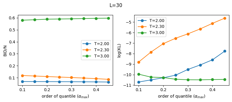
\(r_{max}\) dependence
We cannot fit a bimodal histogram with our unimodal Ansatz, Eq. (2), so one way to proceed is to make a local fit of the first part of each histogram using the meta-parameter \(\alpha_{max}\) defined in Eq. (5). Note that any \(\alpha_{max} < \frac{1}{2}\) will remove the second part of the histogram. Nonetheless \(\alpha_{max}\) is not a parameter of the system, so our results should be independent of it.
Below we show that the BID is approximately independent of the meta-parameter, and moreover this dependency is smaller the larger the system size!
[33]:
T_list = np.array([2,2.3,3]) # list of temperatures
L_list = np.array([30,100])  # list of system-sizes

### OPTIMIZATION PARAMETERS USED FOR THIS EXAMPLE (NEEDED TO LOAD RESULTS)
Nsteps = int(1E6)
delta = 5E-4
seed = 1
alphamin = 0
alphamax_list = np.arange(.1,.45+eps,.05) # orders of quantiles of P(r)

### PLACEHOLDERS
d0_list = np.empty(shape=(len(L_list),
                          len(T_list),
                          len(alphamax_list)
                          ),
)
d1_list = np.empty(shape=d0_list.shape)
rmax_list = np.empty(shape=d0_list.shape) # r^* in the paper
logKL_list = np.empty(shape=d0_list.shape)

for L_id,L in enumerate(L_list):
  for T_id,T in enumerate(T_list):
    for alphamax_id,alphamax in enumerate(alphamax_list):
      optfolder0 = f'datasets/hamming/Ising2D/opt/L{L}/T{T:.2f}/' # folder to put results
      B = BID(
              alphamin=alphamin,
              alphamax=alphamax,
              seed=seed,
              delta=delta,
              Nsteps=Nsteps,
              optfolder0=optfolder0
              )
      (rmax_list[L_id,T_id,alphamax_id], # r^* in the paper
      d0_list[L_id,T_id,alphamax_id],    # BID
      d1_list[L_id,T_id,alphamax_id],    # the second variational parameter
      logKL_list[L_id,T_id,alphamax_id], # logarithm of the KL divergence after optimization
      ) = B.load_results()
[34]:
for L_id, L in enumerate(L_list):
  fig, axs = plt.subplots(nrows=1, ncols=2, figsize=(8,3.5))
  ax0, axkl = axs
  for T_id,T in enumerate(T_list):
    lbl = f'{T=:.2f}'
    ax0.plot(alphamax_list,
            d0_list[L_id,T_id,:]/L**2,
            'o-',
            label=lbl,
            )
    axkl.plot(alphamax_list,
            logKL_list[L_id,T_id,:],
            'o-',
            label=lbl,
            )
  ax0.set_ylabel(f"BID/N")
  ax0.set_xlabel(r'order of quantile ($\alpha_{max})$')
  ax0.legend()

  axkl.set_ylabel(f"log(KL)")
  axkl.set_xlabel(r'order of quantile ($\alpha_{max}$)')
  axkl.legend()

  fig.suptitle(f'{L=}')
  plt.tight_layout()
  plt.show()
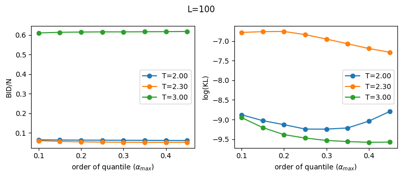
Note:
When studying the BID dependence with system parameters (e.g. here temperature or size), we fix the same \(\alpha_{max}\) for all calculations. \(r_{max}\) can be completely different when varying the system parameters, and \(\alpha_{max}\) allows to select a \(r_{max}\) adaptively and automatically.
Close to \(T_c\) the small size system (\(L=30\)) has a higher KL divergence for larger scales (\(\alpha_{max}\) close to \(\frac{1}{2}\)), where the corresponding histogram has a significant superposition of the two peaks that our model cannot fit. Nonetheless the dependence of the BID with \(\alpha_{max}\) is very mild. Here any \(\alpha_{max}<1/4\) is a safe choice. For \(L=100\) we see that any choice of \(\alpha_{max}\) is fine (in which case taking the biggest seems natural, since we fit more data).
If \(\alpha_{max}\) is too small (say, less than \(0.1\)) then we throw away almost all data. We would be fitting the initial part of the histogram than can be noisy or not statistically relevant for the problem. For example, In dynamical systems we observe that temporal autocorrelations produce long tails on the left part of the histogram (work in progress), which are physically meaningless.
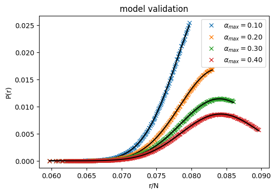
Model validation
In continuous black line the model prediction, in colors the empirical probabilities.
Note that each histogram is cut at some \(r_{max}\) depending on the chosen value of \(\alpha_{max}\), and re-normalize by the total number of counts in that regime.
You can see what happens with other temperatures like 1.5, 1.6, 1.7, … ,4 and or L = 30.
[35]:
T = 2
L = 100
N = L**2
alphamax_list = np.arange(.1,.4+eps,.1) # orders of quantiles of P(r)

fig,ax = plt.subplots(1,figsize=(6,4))
for alphamax_id,alphamax in enumerate(alphamax_list):
  optfolder0 = f'datasets/hamming/Ising2D/opt/L{L}/T{T:.2f}/' # folder to put results
  B = BID(
          alphamin=alphamin,
          alphamax=alphamax,
          seed=seed,
          delta=delta,
          Nsteps=Nsteps,
          optfolder0=optfolder0
          )
  remp,Pemp,Pmodel = B.load_fit()    # to do explicit model validation
  ax.plot(remp/N,Pemp,'x',label=r'$\alpha_{max}=$'+f'{alphamax:.2f}')
  ax.plot(remp/N,Pmodel,'-',color='black')

ax.set_xlabel('r/N')
ax.set_ylabel('P(r)')
plt.title('model validation')
ax.legend()
plt.show()
[ ]: