Tutorial: Differentiable Information Imbalance (JAX implementation)
The Differentiable Information Imbalance (DII) is a tool to automatically learn the optimal distance function A to predict close pair of points in a target distance space B.
This notebook shows a brief tutorial of the JAX implementation of the DII, available in the ‘DiffImbalance’ class. For more information, please refer to the diff_imbalance module in the DADApy documentation: https://dadapy.readthedocs.io/en/latest/modules.html
[1]:
from dadapy import DiffImbalance
import matplotlib.pyplot as plt
import numpy as np
import os
import jax

jax.config.update("jax_platform_name", "cpu")  # can run on 'cpu' or 'gpu'; restart the
                                               # notebook kernel to make this change effective
os.environ["XLA_PYTHON_CLIENT_PREALLOCATE"] = "false"  # avoid jax memory preallocation
[2]:
%load_ext autoreload
%autoreload 2
Optimization on a 5D anisotropic Gaussian dataset
The differentiable Information Imbalance is computed here as \begin{equation} DII(d^A(\boldsymbol{w})\rightarrow B) = \frac{2}{N^2} \sum_{i,j=1}^N\, c_{ij}^A\, r_{ij}^B\, \hspace{1cm} \Bigg( c_{ij}^A = \frac{\exp(-d_{ij}^A(\boldsymbol{w})^2/\lambda)}{\sum_{k(\neq i)}{\exp(-d_{ik}^A(\boldsymbol{w})^2/\lambda)}}\Bigg). \end{equation} Qualitatively, parameter \(\lambda\) decides how many neighbors are considered - for very small \(\lambda\), only the neigherest neighbor receives a weight of \(~1\), and all other neighbors receive weights close to \(0\).
In this example we show how to assign the optimal weights \(\boldsymbol{w} = \{w_\alpha\}\) to the features \(\{X_\alpha\}\) \((\alpha=1,...,D)\), which define space A, in order to optimize the prediction of distances in a target space B. We will construct space A using a 5-dimensional isotropic Gaussian distribution, and space B by reweighting its coordinates, resulting in a 5-dimensional anisotropic Gaussian.
The weights appear in the distance function as \begin{equation} d_{ij}^A(\boldsymbol{w}) = \Bigg[\sum_{\alpha=1}^D\,(w_{\alpha}X_\alpha^i - w_{\alpha}X_\alpha^j)^2 \Bigg]^{1/2}, \end{equation} and they are optimized by gradient descent.
[3]:
# generate test data
weights_ground_truth = np.array([10, 3, 1, 30, 7.3])
np.random.seed(0)
data_A = np.random.normal(loc=0, scale=1.0, size=(500, 5))  # sample 500 points
data_B = weights_ground_truth[np.newaxis, :] * data_A

# train the DII to recover ground-truth metric
dii = DiffImbalance(
    data_A=data_A,  # matrix of shape (N,D_A)
    data_B=data_B,  # matrix of shape (N,D_B)
    periods_A=None,
    periods_B=None,
    seed=0,
    num_epochs=500,
    batches_per_epoch=1,  # no mini-batches
    l1_strength=0.0,  # no l1 regularization
    point_adapt_lambda=True,
    k_init=1,
    k_final=1,
    params_init=None,  # automatically set to [0.1,0.1,0.1,0.1,0.1]
    optimizer_name="sgd",  # possible choices: "sgd", "adam", "adamw"
    learning_rate=1e-2,
    learning_rate_decay=None,  # possible choices: None, "cos", "exp"
    num_points_rows=None,
)
weights, imbs = dii.train()

print(f"Ground truth weights = {weights_ground_truth}\n")
# scale learnt weights in same range of ground-truth ones (same magnitude of the largest one)
print(
    f"Learnt weights: {np.abs(weights[-1]) / (np.max(np.abs(weights[-1])) / np.max(weights_ground_truth))}"
)
Ground truth weights = [10.   3.   1.  30.   7.3]

Learnt weights: [ 9.99  2.95  0.89 30.    7.31]
[4]:
# plot the DII and the weights during the training
fig, (ax1, ax2) = plt.subplots(1, 2, figsize=(12, 4))
ax1.plot(imbs)
ax2.plot(weights[:, 0], label="$w_1$")
ax2.plot(weights[:, 1], label="$w_2$")
ax2.plot(weights[:, 2], label="$w_3$")
ax2.plot(weights[:, 3], label="$w_4$")
ax2.plot(weights[:, 4], label="$w_5$")

ax1.set(ylabel="Differentiable Information Imbalance", xlabel="Epoch number")
ax2.set(ylabel="Weights", xlabel="Epoch number")
ax2.legend()
plt.show()
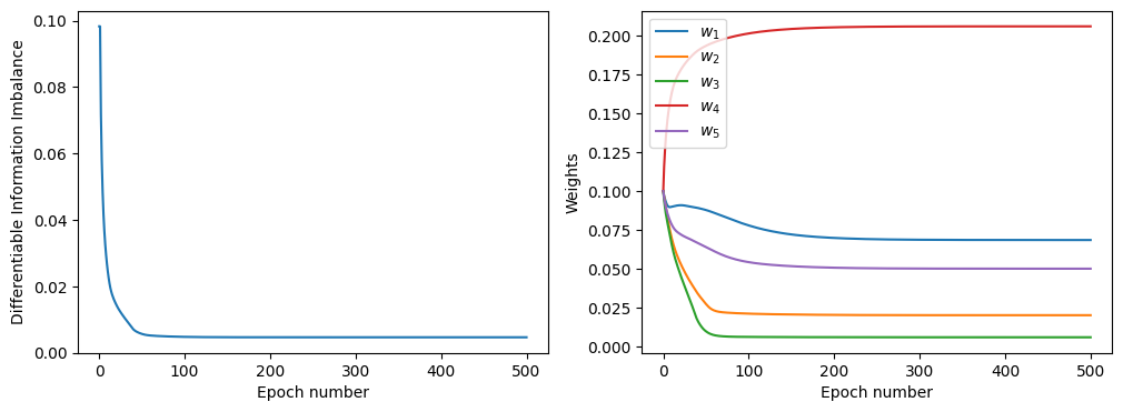
The plots above show the convergence of the DII (left panel) and of the feature weights (right panel) as a function of the epoch number.
In this simple example we employed no decay schedule for the learning rate (argument ‘learning_rate_decay’), although possible options are ‘cos’ (cosine decay) and ‘exp’ (learning rate is halved every 10 epochs). Although these schedules avoid “overshooting” the minimum and can improve the optimization of the DII, we suggest to always perform a first optimization in absence of any learning rate decay schedule, to verify that the number of epoches (argument ‘num_epochs’) is appropriate to ensure convergence.
In particularly noisy data sets, strategies to speed up and improve the DII optimization include the use of mini-batches (argument ‘batches_per_epoch’) coupled with more sophisticated optimizers (e.g. ‘adam’), and the use of a larger neighborhood size for setting the parameter \(\lambda\) adaptively (arguments ‘k_init’ and ‘k_final’). Viable options are setting ‘batches_per_epoch’ such that each mini-batch contains ~100 points, and setting ‘k_init’ and ‘k_final’ such that ~5% of the points are included in each neighborhood. For example, if the original data set contains \(N=500\) points, setting ‘batches_per_epoch’ to 5 results in mini-batches of \(N'=100\) points each, and setting ‘k_init’ and ‘k_final’ to 5 allows selecting 5% of the points in each mini-batch:
[5]:
# train the DII to recover ground-truth metric
dii = DiffImbalance(
    data_A=data_A,  # matrix of shape (N,D_A)
    data_B=data_B,  # matrix of shape (N,D_B)
    periods_A=None,
    periods_B=None,
    seed=0,
    num_epochs=500,
    batches_per_epoch=5,  # no mini-batches
    l1_strength=0.0,  # no l1 regularization
    point_adapt_lambda=True,
    k_init=5,
    k_final=5,
    params_init=None,  # automatically set to [0.1,0.1,0.1,0.1,0.1]
    optimizer_name="adam",  # possible choices: "sgd", "adam", "adamw"
    learning_rate=1e-2,
    learning_rate_decay="cos",  # possible choices: None, "cos", "exp"
    num_points_rows=None,
)
weights, imbs = dii.train()  # the outputs can also be accessed after training
# with dii.params_training and dii.imbs_training

print(f"Ground truth weights = {weights_ground_truth}\n")

# scale learnt weights in same range of ground-truth ones (same magnitude of the largest one)
print(
    f"Learnt weights: {np.abs(weights[-1]) / (np.max(np.abs(weights[-1])) / np.max(weights_ground_truth))}"
)
Ground truth weights = [10.   3.   1.  30.   7.3]

Learnt weights: [10.04  2.86  0.57 30.    7.3 ]
[6]:
# plot the DII and the weights during the training
fig, (ax1, ax2) = plt.subplots(1, 2, figsize=(12, 4))
ax1.plot(imbs)
ax2.plot(weights[:, 0], label="$w_1$")
ax2.plot(weights[:, 1], label="$w_2$")
ax2.plot(weights[:, 2], label="$w_3$")
ax2.plot(weights[:, 3], label="$w_4$")
ax2.plot(weights[:, 4], label="$w_5$")

ax1.set(ylabel="Differentiable Information Imbalance", xlabel="Epoch number")
ax2.set(ylabel="Weights", xlabel="Epoch number")
ax2.legend()
plt.show()
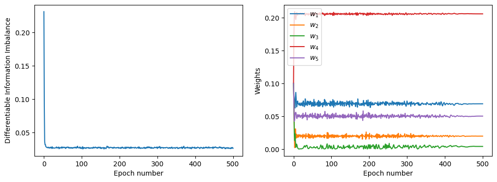
In this case, the panel on the left depicts the DII computed, at each training epoch, over the last mini-batch employed in that epoch. The DII can be computed on the full data set after convergence using the method ‘return_final_dii’. For details on its arguments refer to the DADApy documentation: https://dadapy.readthedocs.io/en/latest/modules.html.
[7]:
imb_final, _ = dii.return_final_dii(
    compute_error=False, ratio_rows_columns=None, seed=0, discard_close_ind=0
)
print(f"Optimal DII over full data set: {imb_final:2f}")  # can also be accessed
# through dii.imb_final
Optimal DII over full data set: 0.011225
Greedy Feature Search: Forward Search Implementation
Feature selection can be achieved either by optimizing the DII with a L1 regularization, or with a greedy search approach. We show in this section how to run a “forward” greedy search, where we first identify the optimal single feature and successively add features one by one to get the optimal n-tuple feature sets. The process is called “greedy” because it does not explore every possible combination of features, since that would be computationally untenable for high-dimensional datasets.
The parameter n_best controls the greediness of the algorithm. If n_best is set to 1, the optimal n-tuple is identified by adding one feature at a time to the optimal (n-1)-tuple (by only adding features that are not already contained in this (n-1)-tuple). The candidate n-tuples are optimized according to the DII, and the one providing the lowest DII is selected for the next step. If n_best is not 1, the optimal n-tuple is identified by adding one feature at a time to the optimal
n_best tuples of size (n-1), resulting in a broader exploration of the search space at the price of an increased runtime.
In the following example, we use the same 5-dimensional Gaussian of the previous tests, with ground-trith weights [10, 3, 1, 30, 7.3]. Hence, the optimal n-tuples for each value of n should be:
n=1 -> [3]
n=2 -> [0, 3]
n=3 -> [0, 3, 4]
n=4 -> [0, 1, 3, 4]
n=5 -> [0, 1, 2, 3, 4]
The “forward” greedy search is the recommended approach to use when one is looking to select few relevant features (compared to the total possible number of features).
[8]:
# initialize DII object
dii = DiffImbalance(
    data_A,
    data_B,
    periods_A=None,
    periods_B=None,
    seed=0,
    num_epochs=50,
    batches_per_epoch=5,
    l1_strength=0.0,
    point_adapt_lambda=True,
    k_init=5,
    k_final=5,
    lambda_factor=1e-1,
    params_init=None,
    optimizer_name="sgd",
    learning_rate=1e-1,
    learning_rate_decay="cos",
    num_points_rows=None,
)
[9]:
# forward greedy search
(
    feature_sets_fw,
    diis_fw,
    errors_fw,
    weights_fw,
) = dii.forward_greedy_feature_selection(
    n_features_max=5,
    n_best=10,
    compute_error=True,
    ratio_rows_columns=1,
    seed=0,
    discard_close_ind=0,
)

diis_fw_array = np.array(diis_fw)
Feature set = [0], DII = 0.8999369144439697
Feature set = [1], DII = 0.9869815111160278
Feature set = [2], DII = 0.9980540871620178
Feature set = [3], DII = 0.24966953694820404
Feature set = [4], DII = 0.9708154201507568

------------------------------------------------
Best single feature: [3]
        DII: 0.24966953694820404
        Optimal weights: [0.  0.  0.  0.1 0. ]
Selected 5 best candidates for next iteration
------------------------------------------------
Feature set = [0, 3], DII = 0.09266918152570724
Feature set = [1, 3], DII = 0.23958951234817505
Feature set = [2, 3], DII = 0.246477410197258
Feature set = [3, 4], DII = 0.1784021258354187
Feature set = [0, 1], DII = 0.8793059587478638
Feature set = [0, 2], DII = 0.8912973999977112
Feature set = [0, 4], DII = 0.8359236121177673
Feature set = [1, 4], DII = 0.9284022450447083
Feature set = [2, 4], DII = 0.965333878993988
Feature set = [1, 2], DII = 0.9652037620544434
Optimal weights for feature set [0, 3]: [0.04 0.   0.   0.13 0.  ]

------------------------------------------------
Best 2-tuple: [0, 3]
        DII: 0.09266918152570724
        Optimal weights: [0.04 0.   0.   0.13 0.  ]
Selected 10 best candidates for next iteration
------------------------------------------------
Feature set = [0, 1, 3], DII = 0.07907145470380783
Feature set = [0, 2, 3], DII = 0.09184076637029648
Feature set = [0, 3, 4], DII = 0.025932027027010918
Feature set = [1, 3, 4], DII = 0.1665874570608139
Feature set = [2, 3, 4], DII = 0.18107758462429047
Feature set = [1, 2, 3], DII = 0.24252423644065857
Feature set = [0, 1, 4], DII = 0.8256341218948364
Feature set = [0, 2, 4], DII = 0.8317562937736511
Feature set = [0, 1, 2], DII = 0.8771141767501831
Feature set = [1, 2, 4], DII = 0.9303593635559082
Optimal weights for feature set [0, 3, 4]: [0.05 0.   0.   0.16 0.04]

------------------------------------------------
Best 3-tuple: [0, 3, 4]
        DII: 0.025932027027010918
        Optimal weights: [0.05 0.   0.   0.16 0.04]
Selected 10 best candidates for next iteration
------------------------------------------------
Feature set = [0, 1, 3, 4], DII = 0.02279951423406601
Feature set = [0, 2, 3, 4], DII = 0.02594083920121193
Feature set = [0, 1, 2, 3], DII = 0.07834427058696747
Feature set = [1, 2, 3, 4], DII = 0.1662881225347519
Feature set = [0, 1, 2, 4], DII = 0.8106766939163208
Optimal weights for feature set [0, 1, 3, 4]: [0.06 0.02 0.   0.18 0.05]

------------------------------------------------
Best 4-tuple: [0, 1, 3, 4]
        DII: 0.02279951423406601
        Optimal weights: [0.06 0.02 0.   0.18 0.05]
Selected 5 best candidates for next iteration
------------------------------------------------
Feature set = [0, 1, 2, 3, 4], DII = 0.02285277657210827
Optimal weights for feature set [0, 1, 2, 3, 4]: [0.07 0.02 0.   0.21 0.05]

------------------------------------------------
Best 5-tuple: [0, 1, 2, 3, 4]
        DII: 0.02285277657210827
        Optimal weights: [0.07 0.02 0.   0.21 0.05]
Selected 1 best candidates for next iteration
------------------------------------------------
[10]:
print(f"\nSelected feature subsets:\n {feature_sets_fw}\n")
print("Forward DIIs:", diis_fw)
print("Forward Errors:", errors_fw)
print("Forward Weights:", weights_fw)

print("\nOriginal weights:", weights_ground_truth)
print(
    f"\nLearnt weights for the full feature space: {np.abs(weights_fw[-1]) / (np.max(np.abs(weights_fw[-1])) / np.max(weights_ground_truth))}"
)
print(
    f"\nAll weights along the feature selection:\n {np.abs(weights_fw) / (np.max(np.abs(weights_fw)) / np.max(weights_ground_truth))}"
)
Selected feature subsets:
 [[3], [0, 3], [0, 3, 4], [0, 1, 3, 4], [0, 1, 2, 3, 4]]

Forward DIIs: [0.24966953694820404, 0.09266918152570724, 0.025932027027010918, 0.02279951423406601, 0.02285277657210827]
Forward Errors: [0.007513741031289101, 0.005023834761232138, 0.000543437316082418, 0.00034482675255276263, 0.0003450679068919271]
Forward Weights: [array([0. , 0. , 0. , 0.1, 0. ]), array([0.04, 0.  , 0.  , 0.13, 0.  ], dtype=float32), array([0.05, 0.  , 0.  , 0.16, 0.04], dtype=float32), array([0.06, 0.02, 0.  , 0.18, 0.05], dtype=float32), array([0.07, 0.02, 0.  , 0.21, 0.05], dtype=float32)]

Original weights: [10.   3.   1.  30.   7.3]

Learnt weights for the full feature space: [10.17  2.78  0.6  30.    7.39]

All weights along the feature selection:
 [[ 0.    0.    0.   14.6   0.  ]
 [ 6.27  0.    0.   19.68  0.  ]
 [ 7.88  0.    0.   23.32  5.82]
 [ 9.09  2.48  0.   26.84  6.63]
 [10.17  2.78  0.6  30.    7.39]]
Greedy Feature Search: Backward Search Implementation
Here we implement the “backward” greedy search approach, starting with all the features and then successively removing features one by one to get the most optimal n-plet feature sets. As in the “forward” greedy search implementation, the parameter n_best controls the greediness of the algorithm. If n_best is set to 1, the optimal n-tuple is identified by removing one feature at a time to the optimal (n+1)-tuple (by only adding features that are not already contained in this
(n+1)-tuple). The candidate n-tuples are optimized according to the DII, and the one providing the lowest DII is selected for the next step. If n_best is not 1, the optimal n-tuple is identified by removing one feature at a time to the n_best optimal tuples of size (n+1).
In the following example, the optimal n-plets for each value of n should be:
n=5 -> [0, 1, 2, 3, 4]
n=4 -> [0, 1, 3, 4]
n=3 -> [0, 3, 4]
n=2 -> [0, 3]
n=1 -> [3]
The “backward” greedy search is the recommended approach to use when one is looking to select a significant number of relevant features (compared to the total possible number of features), or a case where one just wants to eliminate a few uninformative features.
[11]:
# initialize DII object and train over full feature space
dii = DiffImbalance(
    data_A,
    data_B,
    periods_A=None,
    periods_B=None,
    seed=0,
    num_epochs=50,
    batches_per_epoch=5,
    l1_strength=0.0,
    point_adapt_lambda=True,
    k_init=5,
    k_final=5,
    lambda_factor=1e-1,
    params_init=None,
    optimizer_name="sgd",
    learning_rate=1e-1,
    learning_rate_decay="cos",
    num_points_rows=None,
)
weights, imbs = dii.train()
[12]:
# forward greedy selection
(
    feature_sets_bw,
    diis_bw,
    errors_bw,
    weights_bw,
) = dii.backward_greedy_feature_selection(
    n_features_min=1,
    n_best=10,
    compute_error=True,
    ratio_rows_columns=1,
    seed=0,
    discard_close_ind=0,
)

diis_bw_array = np.array(diis_bw)
------------------------------------------------
All features: [[0, 1, 2, 3, 4]]
        DII: 0.022820621728897095
        Optimal weights: [0.07 0.02 0.   0.21 0.05]
------------------------------------------------
Feature set = [1, 2, 3, 4], DII = 0.16653390228748322
Feature set = [0, 2, 3, 4], DII = 0.02594083920121193
Feature set = [0, 1, 3, 4], DII = 0.022799985483288765
Feature set = [0, 1, 2, 4], DII = 0.8058949112892151
Feature set = [0, 1, 2, 3], DII = 0.0787024274468422
------------------------------------------------
Best 4-tuple: [0, 1, 3, 4]
        DII: 0.022799985483288765
        Optimal weights: [0.06 0.02 0.   0.18 0.05]
Selected 5 best candidates for next iteration
------------------------------------------------
Feature set = [1, 3, 4], DII = 0.1665170043706894
Feature set = [0, 3, 4], DII = 0.0259428508579731
Feature set = [0, 1, 4], DII = 0.8102166056632996
Feature set = [0, 1, 3], DII = 0.07857366651296616
Feature set = [2, 3, 4], DII = 0.18107758462429047
Feature set = [0, 2, 4], DII = 0.8303636908531189
Feature set = [0, 2, 3], DII = 0.09187900274991989
Feature set = [1, 2, 3], DII = 0.23959513008594513
Feature set = [0, 1, 2], DII = 0.8771141767501831
Feature set = [1, 2, 4], DII = 0.9303593635559082
------------------------------------------------
Best 3-tuple: [0, 3, 4]
        DII: 0.0259428508579731
        Optimal weights: [0.05 0.   0.   0.16 0.04]
Selected 10 best candidates for next iteration
------------------------------------------------
Feature set = [3, 4], DII = 0.17846915125846863
Feature set = [0, 4], DII = 0.8343183994293213
Feature set = [0, 3], DII = 0.0921807810664177
Feature set = [1, 3], DII = 0.2390105277299881
Feature set = [0, 1], DII = 0.8793059587478638
Feature set = [2, 3], DII = 0.24573972821235657
Feature set = [0, 2], DII = 0.898990273475647
Feature set = [1, 4], DII = 0.9284022450447083
Feature set = [2, 4], DII = 0.965333878993988
Feature set = [1, 2], DII = 0.9652037620544434
------------------------------------------------
Best 2-tuple: [0, 3]
        DII: 0.0921807810664177
        Optimal weights: [0.04 0.   0.   0.13 0.  ]
Selected 10 best candidates for next iteration
------------------------------------------------
Feature set = [3], DII = 0.24966953694820404
Feature set = [0], DII = 0.8999369144439697
Feature set = [4], DII = 0.9708154201507568
Feature set = [1], DII = 0.9869815111160278
Feature set = [2], DII = 0.9980540871620178
------------------------------------------------
Best 1-tuple: [3]
        DII: 0.24966953694820404
        Optimal weights: [0.  0.  0.  0.1 0. ]
Selected 5 best candidates for next iteration
------------------------------------------------
[13]:
print(f"\nSelected feature subsets:\n {feature_sets_bw}\n")

print("Backward DIIs:", diis_bw)
print("Backward Errors:", errors_bw)
print("Backward Weights:", weights_bw)

print("\nOriginal weights:", weights_ground_truth)
print(
    f"\nLearnt weights for the full feature space: {np.abs(weights_bw[0]) / (np.max(np.abs(weights_bw[0])) / np.max(weights_ground_truth))}"
)
print(
    f"\nAll weights along the feature selection:\n {np.abs(weights_bw) / (np.max(np.abs(weights_bw)) / np.max(weights_ground_truth))}"
)
Selected feature subsets:
 [[0, 1, 2, 3, 4], [0, 1, 3, 4], [0, 3, 4], [0, 3], [3]]

Backward DIIs: [0.022820621728897095, 0.022799985, 0.02594285, 0.09218078, 0.24966954]
Backward Errors: [0.0003439213614910841, 0.00034475446, 0.0005474837, 0.004991478, 0.007513741]
Backward Weights: [Array([0.07, 0.02, 0.  , 0.21, 0.05], dtype=float32), Array([0.06, 0.02, 0.  , 0.18, 0.05], dtype=float32), Array([0.05, 0.  , 0.  , 0.16, 0.04], dtype=float32), Array([0.04, 0.  , 0.  , 0.13, 0.  ], dtype=float32), Array([0. , 0. , 0. , 0.1, 0. ], dtype=float32)]

Original weights: [10.   3.   1.  30.   7.3]

Learnt weights for the full feature space: [10.17  2.78  0.6  30.    7.39]

All weights along the feature selection:
 [[10.17  2.78  0.6  30.    7.39]
 [ 9.09  2.48  0.   26.84  6.63]
 [ 7.88  0.    0.   23.32  5.82]
 [ 6.27  0.    0.   19.68  0.  ]
 [ 0.    0.    0.   14.6   0.  ]]