Tutorial: Differentiable Information Imbalance
The Differentiable Information Imbalance (DII) is used to select and optimally scale features (variables) to be informative of about a ground truth.
DII is implemented in the ‘FeatureWeighting’ class. To see all the functions that you can call within this class, please refer to: The feature_weighting module in the DADApy documentation: https://dadapy.readthedocs.io/en/latest/modules.html
[1]:
import matplotlib.pyplot as plt
import numpy as np
from itertools import combinations_with_replacement

from dadapy.metric_comparisons import MetricComparisons
from dadapy.feature_weighting import FeatureWeighting

%matplotlib inline
[2]:
%load_ext autoreload
%autoreload 2
Comparison with the standard Information Imbalance
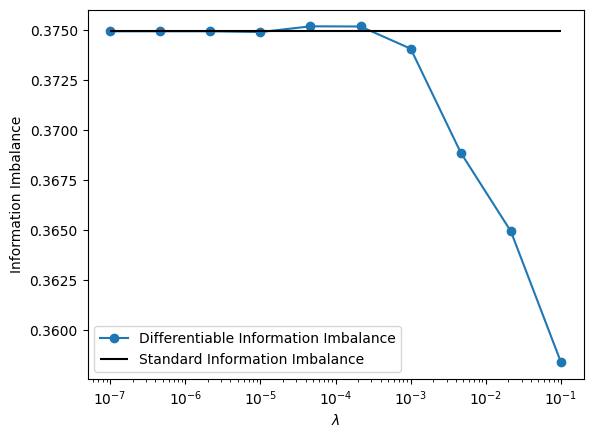
In this section we show how to compute the differentiable Information Imbalance, \begin{equation} DII(A\rightarrow B) = \frac{2}{N^2} \sum_{i,j=1}^N\, c_{ij}^A\, r_{ij}^B\, \hspace{1cm} \Bigg( c_{ij}^A = \frac{\exp(-d_{ij}^A/\lambda)}{\sum_{k(\neq i)}{\exp(-d_{ik}^A/\lambda)}}\Bigg), \end{equation} for different choices of the softmax parameter \(\lambda\), and we see that the differentiable version tends to the standard Information Imbalance in the limit of small \(\lambda\). Qualitatively, this parameter decides how many neighbors are considered - for very small \(\lambda\), only the neigherest neighbor receives a weight of \(~1\), all other neighbors weights close to \(0\). We will define the distance spaces A and B using subsets of coordinates from a isotropic 3D Gaussian distribution.
Included methods:
Prediction of distance space B from distance space A for a given value of \(\lambda\): return_dii
[3]:
# sample dataset
N = 1000
cov = np.identity(3)
mean = np.zeros(3)
np.random.seed(9)
X = np.random.multivariate_normal(mean=mean, cov=cov, size=(N))

# define spaces A and B by subsets of coordinates
coords1 = [0, 1]
coords2 = [0, 1, 2]
[4]:
# define an instance of the FeatureWeighting class
f = FeatureWeighting(coordinates=X[:, coords1])
f_target = FeatureWeighting(coordinates=X[:, coords2])

diff_imbs = []
lambdas = np.logspace(-7, -1, 10)  # uniformly spaced in [1e-7, 1e-1] in log scale
for lambd in lambdas:
    diff_imbs.append(f.return_dii(target_data=f_target, lambd=lambd))
/var/folders/gs/c6kntl8s5z7b8jcdsd9xydww0000gp/T/ipykernel_64904/1281833669.py:8: UserWarning: maxk option not yet available for the FeatureWeighting class. It will be set to the number of data-1 (1000-1).
  diff_imbs.append(f.return_dii(target_data=f_target, lambd=lambd))
We compute for comparison purposes the standard Information Imbalance between the same distance spaces:
[5]:
# define an instance of the MetricComparisons class
d = MetricComparisons(X, maxk=N - 1)
imbs = d.return_inf_imb_two_selected_coords(coords1=coords1, coords2=coords2)
[6]:
plt.plot(lambdas, diff_imbs, "o-", label="Differentiable Information Imbalance")
plt.hlines(
    imbs[0],
    lambdas[0],
    lambdas[-1],
    color="black",
    label="Standard Information Imbalance",
)
plt.xscale("log")
plt.xlabel("$\\lambda$")
plt.ylabel("Information Imbalance")
plt.legend()
plt.show()
Optimization on a 10D anisotropic Gaussian dataset
In this example we show how to optimize the weights \(\{w_\alpha\}\) of the features \(\{X_\alpha\}\) in a space A \((\alpha=1,...,D)\) in order to optimize the prediction of the distances measured in a target space B. We will construct space A using a 10D isotropic Gaussian distribution, and space B by reweighting its coordinates, resulting in a 10D anisotropic Gaussian.
The weights appear in the distance function as \begin{equation} d_{ij}^A(\{w_\alpha\}) = \Bigg[\sum_{\alpha=1}^D\,(w_{\alpha}X_\alpha^i - w_{\alpha}X_\alpha^j) \Bigg]^{1/2} \end{equation}
Included methods:
Gradient-descent optimization of the DII with respect to weights of features in space A, given a target distance space B: return_weights_optimize_dii
[3]:
# sample datasets
N = 500  # number of points
d = 10  # dimension

cov = np.identity(10)
mean = np.zeros(10)
X = np.random.multivariate_normal(mean=mean, cov=cov, size=(N))  # isotropic Gaussian

weights = np.ones(10) * (0.01**2)
weights[0:5] = [5, 2, 1, 1, 0.5]
X_target = X * weights  # target space B constructed on this anisotropic Gaussian
The following block carries out the optimization:
[8]:
n_epochs = 50  # number of training epochs

f = FeatureWeighting(coordinates=X)
f_target = FeatureWeighting(coordinates=X_target)
final_weights = f.return_weights_optimize_dii(
    target_data=f_target,
    initial_weights=None,  # (default) automatic weights as inverse std.dev. of features
    n_epochs=n_epochs,
)
/home/romi/anaconda3/lib/python3.7/site-packages/ipykernel_launcher.py:7: UserWarning: maxk option not yet available for the FeatureWeighting class. It will be set to the number of data-1 (500-1).
  import sys
If the arguments ‘lambd’ and ‘learning_rate’ are not specified, these parameters are set automatically. After the optimization the FeatureWeighting object allows to access the values of the DII and the weights during the training, using the history:
[9]:
dii_per_epoch = f.history["dii_per_epoch"]
weights_per_epoch = f.history["weights_per_epoch"]

fig, (ax1, ax2) = plt.subplots(1, 2, figsize=(10, 4))
ax1.plot(np.arange(n_epochs + 1), dii_per_epoch)
ax2.plot(np.arange(n_epochs + 1), weights_per_epoch[:, 0], label="$w_1$")
ax2.plot(np.arange(n_epochs + 1), weights_per_epoch[:, 1], label="$w_2$")
ax2.plot(np.arange(n_epochs + 1), weights_per_epoch[:, 2], label="$w_3$")

ax1.set(ylabel="Differentiable Information Imbalance", xlabel="Epoch number")
ax2.set(ylabel="Sample weights", xlabel="Epoch number")
ax2.legend()
plt.show()
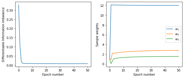
We can visually compare the ground-truth weights of the anisotropic 10D Gaussian (i.e. the marginal standard deviations of the coordinates) and the optimal weights obtained from the optimization, after scaling them in the range [0,1]:
[8]:
weights_names = (
    "$w_1$",
    "$w_2$",
    "$w_3$",
    "$w_4$",
    "$w_5$",
    "$w_6$",
    "$w_7$",
    "$w_8$",
    "$w_9$",
    "$w_{10}$",
)
weights_grouped = {
    "Ground-truth weights": weights / max(weights),
    "Learnt weights (DII)": final_weights / max(final_weights),
}

x = np.arange(len(weights_names))  # label locations
width = 0.2  # bar widths
multiplier = 0

fig, ax = plt.subplots()
for attribute, measurement in weights_grouped.items():
    offset = width * multiplier
    ax.bar(x + offset, measurement, width, label=attribute, edgecolor="white")
    multiplier += 1

ax.set_ylabel("Weights (scaled in range [0,1])")
ax.set_xticks(x + width, weights_names)
ax.legend()
plt.show()

From the bar plot above we see that the scaled weights reproduce well the target standard deviations of the anisotropic Gaussian distribution
Backward greedy elimination
Backward greedy elimination is an efficient heuristic for selectin smaller features sets, given \(\leq\) 100 input features.
In this example we illustrate, given a target space B and a starting set of \(D\) candidate features in space A, all the optimal subsets of \(D' (\leq D)\) features to predict B are identified. At each step, the weights of the candidate features are optimized by minimizing the DII to the target space B, and after each optimization the feature associated to the lowest weight is discarded. The search stops when the optimal subset with a single feature is identified.
For space A we employ 65 candidate features, given by all the monomials of degree up to 2 obtained from a set of 10 independent Gaussian features of zero mean and unit variance (\(x_i \sim \mathcal{N}(0,1)\)): \begin{equation} \underbrace{x_1, x_2, ...}_{\text{order 1}},\, \underbrace{x_1^2, x_2^2, ..., x_1\,x_2,\, x_1\,x_3, ...}_{\text{order 2}}\,. \end{equation} The target distance B is constructed by selecting with different weights only 10 of the 65 monomials.
Included methods:
Stepwise backward greedy elimination: return_backward_greedy_dii_elimination
[11]:
# create all subsets of 10 elements with cardinality 1 or 2
ncoords = range(10)
monomials_list = []
for degree in [1, 2]:
    monomials_list += list(combinations_with_replacement(ncoords, degree))

# use subsets to construct all possible monomials up to degree 2
X_monomials = np.empty((X.shape[0], len(monomials_list)))
for i_monomial, coords in enumerate(monomials_list):
    monomial = np.prod(X[:, coords], axis=1)
    X_monomials[:, i_monomial] = monomial
[12]:
# construct the target space B by selecting 10 monomials with different weights
monomials_target = [5, 8, 12, 14, 20, 26, 35, 47, 59, 61]
weights = np.zeros(len(monomials_list))
weights[monomials_target] = [5, 5, 7, 2, 1, 4, 1.5, 1, 3, 6]

coords_names = np.array(
    ["X_1", "X_2", "X_3", "X_4", "X_5", "X_6", "X_7", "X_8", "X_9", "X_{10}"]
)
print("Selected monomials in target space B:")
for monomial_index in monomials_target:
    monomial = monomials_list[monomial_index]
    print(f"\t{coords_names[list(monomial)]} with weight {weights[monomial_index]}")

X_monomials_target = X_monomials * weights
Selected monomials in target space B:
        ['X_6'] with weight 5.0
        ['X_9'] with weight 5.0
        ['X_1' 'X_3'] with weight 7.0
        ['X_1' 'X_5'] with weight 2.0
        ['X_2' 'X_2'] with weight 1.0
        ['X_2' 'X_8'] with weight 4.0
        ['X_3' 'X_9'] with weight 1.5
        ['X_5' 'X_8'] with weight 1.0
        ['X_8' 'X_8'] with weight 3.0
        ['X_8' 'X_{10}'] with weight 6.0
The following block carries out the backward elimination starting from the whole space of the 65 features (monomials) in space A. This calculation might take ~20 min on a standard laptop; the progression state can be monitored by setting verbose=True when the FeatureWeighting object is initialized.
[14]:
n_epochs = 80  # number of training epochs

f = FeatureWeighting(coordinates=X_monomials, verbose=True)
f_target = FeatureWeighting(coordinates=X_monomials_target)

final_imbs, final_weights = f.return_backward_greedy_dii_elimination(
    target_data=f_target,
    initial_weights=None,  # set automatically (default)
    n_epochs=n_epochs,
    learning_rate=None,  # set automatically (default)
)
/home/romi/anaconda3/lib/python3.7/site-packages/ipykernel_launcher.py:10: UserWarning: maxk option not yet available for the FeatureWeighting class. It will be set to the number of data-1 (500-1).
  # Remove the CWD from sys.path while we load stuff.
number of nonzero weights: 65, execution time: 33.13 s.
number of nonzero weights: 64, execution time: 34.30 s.
number of nonzero weights: 63, execution time: 29.93 s.
number of nonzero weights: 62, execution time: 29.55 s.
number of nonzero weights: 61, execution time: 31.18 s.
number of nonzero weights: 60, execution time: 29.06 s.
number of nonzero weights: 59, execution time: 27.85 s.
number of nonzero weights: 58, execution time: 26.99 s.
number of nonzero weights: 57, execution time: 27.07 s.
number of nonzero weights: 56, execution time: 25.89 s.
number of nonzero weights: 55, execution time: 25.45 s.
number of nonzero weights: 54, execution time: 24.73 s.
number of nonzero weights: 53, execution time: 24.96 s.
number of nonzero weights: 52, execution time: 24.30 s.
number of nonzero weights: 51, execution time: 24.04 s.
number of nonzero weights: 50, execution time: 24.47 s.
number of nonzero weights: 49, execution time: 24.38 s.
number of nonzero weights: 48, execution time: 18.13 s.
number of nonzero weights: 47, execution time: 16.65 s.
number of nonzero weights: 46, execution time: 16.37 s.
number of nonzero weights: 45, execution time: 16.06 s.
number of nonzero weights: 44, execution time: 15.81 s.
number of nonzero weights: 43, execution time: 15.44 s.
number of nonzero weights: 42, execution time: 15.32 s.
number of nonzero weights: 41, execution time: 14.81 s.
number of nonzero weights: 40, execution time: 14.51 s.
number of nonzero weights: 39, execution time: 14.21 s.
number of nonzero weights: 38, execution time: 13.95 s.
number of nonzero weights: 37, execution time: 14.70 s.
number of nonzero weights: 36, execution time: 15.57 s.
number of nonzero weights: 35, execution time: 14.60 s.
number of nonzero weights: 34, execution time: 12.80 s.
number of nonzero weights: 33, execution time: 12.36 s.
number of nonzero weights: 32, execution time: 12.09 s.
number of nonzero weights: 31, execution time: 11.97 s.
number of nonzero weights: 30, execution time: 11.49 s.
number of nonzero weights: 29, execution time: 11.22 s.
number of nonzero weights: 28, execution time: 10.90 s.
number of nonzero weights: 27, execution time: 10.65 s.
number of nonzero weights: 26, execution time: 10.36 s.
number of nonzero weights: 25, execution time: 9.95 s.
number of nonzero weights: 24, execution time: 9.71 s.
number of nonzero weights: 23, execution time: 9.36 s.
number of nonzero weights: 22, execution time: 9.07 s.
number of nonzero weights: 21, execution time: 8.76 s.
number of nonzero weights: 20, execution time: 8.48 s.
number of nonzero weights: 19, execution time: 8.28 s.
number of nonzero weights: 18, execution time: 7.86 s.
number of nonzero weights: 17, execution time: 7.56 s.
number of nonzero weights: 16, execution time: 7.27 s.
number of nonzero weights: 15, execution time: 6.95 s.
number of nonzero weights: 14, execution time: 6.62 s.
number of nonzero weights: 13, execution time: 6.32 s.
number of nonzero weights: 12, execution time: 6.04 s.
number of nonzero weights: 11, execution time: 5.82 s.
number of nonzero weights: 10, execution time: 5.41 s.
number of nonzero weights: 9, execution time: 5.10 s.
number of nonzero weights: 8, execution time: 4.80 s.
number of nonzero weights: 7, execution time: 4.50 s.
number of nonzero weights: 6, execution time: 4.20 s.
number of nonzero weights: 5, execution time: 3.89 s.
number of nonzero weights: 4, execution time: 3.59 s.
number of nonzero weights: 3, execution time: 3.31 s.
number of nonzero weights: 2, execution time: 3.07 s.
number of nonzero weights: 1, execution time: 2.72 s.
[15]:
# optimized information imbalance vs number of non-zero features
plt.plot(np.arange(X_monomials.shape[1], 0, -1), final_imbs, ".-")
plt.xlabel("Number of non-zero features")
plt.ylabel("DII")
plt.yscale("log")
plt.show()
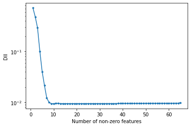
From the plot above we see that the optimized DII reaches a plateau after 9-10 features, which is consistent with the numbers of monomials included in the target space B. We can further verify that, for the subset with 10 non-zero features, both the selected features and their weights are mostly consistent with the ground-truth ones:
[16]:
n_subset = 10
monomials_learnt = np.where(final_weights[-n_subset] > 0)[0]
union_set = list(set(monomials_target).union(monomials_learnt))

weights_grouped = {
    "Ground-truth weights": weights[union_set] / max(weights[union_set]),
    "Learnt weights (DII)": final_weights[-n_subset][union_set]
    / max(final_weights[-n_subset][union_set]),
}
weights_names = []
for monomial_index in union_set:
    monomial = monomials_list[monomial_index]
    weights_names.append(f"$w({''.join((coords_names[list(monomial)]))})$")

x = np.arange(len(weights_names))  # label locations
width = 0.2  # bar widths
multiplier = 0
fig, ax = plt.subplots(figsize=(10, 4))
for attribute, measurement in weights_grouped.items():
    offset = width * multiplier
    ax.bar(x + offset, measurement, width, label=attribute, edgecolor="white")
    multiplier += 1
ax.set_ylabel("Weights (scaled in range [0,1])")
ax.set_xticks(x + width, weights_names)
ax.legend()
plt.show()

L1 regularization (lasso)
If you need to select a small subset of features out of a very large input space (\(\geq\) 100 features), L1 regularization is your friend.
In this section we show how to carry out a selection of optimal subsets of features in space A in order to predict a target space B, by optimizing the Differentiable Information Imbalance with a lasso (L1) regularization. Explicitely, the loss function which is minimized is \begin{equation} \mathcal{L} = DII(A(\{w_\alpha\})\rightarrow B) + \beta \sum_{\alpha=1}^D\, |w_\alpha |\,, \end{equation} where \(\beta\) is the strength of the regularization, which determines the number of non-zero weights. To identify subsets with different numbers of non-zero features, a scan over different values of \(\beta\) is required.
We will use the same dataset of monomials employed in the previous example.
Included methods:
Search of optimal subsets of features by optimizing the DII with different strengths of the L1 regularization term : return_lasso_optimization_dii_search
[4]:
# create all subsets of 10 elements with cardinality 1 or 2
ncoords = range(10)
monomials_list = []
for degree in [1, 2]:
    monomials_list += list(combinations_with_replacement(ncoords, degree))

# use subsets to construct all possible monomials up to degree 2
X_monomials = np.empty((X.shape[0], len(monomials_list)))
for i_monomial, coords in enumerate(monomials_list):
    monomial = np.prod(X[:, coords], axis=1)
    X_monomials[:, i_monomial] = monomial
[5]:
# construct space B by selecting 10 monomials with different weights
monomials_target = [5, 8, 12, 14, 20, 26, 35, 47, 59, 61]
weights = np.zeros(len(monomials_list))
weights[monomials_target] = [5, 5, 7, 2, 1, 4, 1.5, 1, 3, 6]

coords_names = np.array(
    ["X_1", "X_2", "X_3", "X_4", "X_5", "X_6", "X_7", "X_8", "X_9", "X_{10}"]
)
print("Selected monomials in target space B:")
for monomial_index in monomials_target:
    monomial = monomials_list[monomial_index]
    print(f"\t{coords_names[list(monomial)]} with weight {weights[monomial_index]}")

X_monomials_target = X_monomials * weights
Selected monomials in target space B:
        ['X_6'] with weight 5.0
        ['X_9'] with weight 5.0
        ['X_1' 'X_3'] with weight 7.0
        ['X_1' 'X_5'] with weight 2.0
        ['X_2' 'X_2'] with weight 1.0
        ['X_2' 'X_8'] with weight 4.0
        ['X_3' 'X_9'] with weight 1.5
        ['X_5' 'X_8'] with weight 1.0
        ['X_8' 'X_8'] with weight 3.0
        ['X_8' 'X_{10}'] with weight 6.0
The following block optimizes the DII(A:nbsphinx-math:rightarrow `B) with a L:math:`_1 regularization. By default, 10 optimizations for different values of the regularization strength \(\beta\) are carried out. If ‘refine=True’, additional values of \(\beta\) are tested in order to identify more subsets with a different number of non-zero features (This option leads to long calculations when the input feature space is large). Specific values of the parameters \(\beta\) to be tested can be set by the user with the argument ‘l1_penalties’. As in the greedy search algorithm, the progress of the optimization can be monitored by setting verbose=True in the initalization of the FeatureWeighting object.
(This calculation without refinement, can take ~5 min on a starndard laptop)
[7]:
n_epochs = 80  # number of training epochs

f = FeatureWeighting(coordinates=X_monomials, verbose=True)
f_target = FeatureWeighting(coordinates=X_monomials_target)

(
    num_nonzero_features,
    l1_penalties_opt_per_nfeatures,
    dii_opt_per_nfeatures,
    weights_opt_per_nfeatures,
) = f.return_lasso_optimization_dii_search(
    target_data=f_target,
    initial_weights=None,  # (default) set automatically
    n_epochs=n_epochs,
    learning_rate=None,  # (default) set automatically
    refine=False,  # only 10 values of the L1 strength are tested
    plotlasso=True,  # automatically show DII vs number of non-zero features
)
/home/romi/anaconda3/lib/python3.7/site-packages/ipykernel_launcher.py:17: UserWarning: maxk option not yet available for the FeatureWeighting class. It will be set to the number of data-1 (500-1).
10 l1-penalties to test:
optimization with l1-penalty 1 of strength 0 took: 22.20 s.
optimization with l1-penalty 2 of strength 1e-06 took: 27.58 s.
optimization with l1-penalty 3 of strength 3.162e-06 took: 28.33 s.
optimization with l1-penalty 4 of strength 1e-05 took: 21.80 s.
optimization with l1-penalty 5 of strength 3.162e-05 took: 22.88 s.
optimization with l1-penalty 6 of strength 0.0001 took: 18.24 s.
optimization with l1-penalty 7 of strength 0.0003162 took: 11.75 s.
optimization with l1-penalty 8 of strength 0.001 took: 6.44 s.
optimization with l1-penalty 9 of strength 0.003162 took: 4.15 s.
optimization with l1-penalty 10 of strength 0.01 took: 3.68 s.
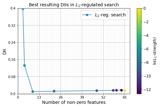
The plot above shows the optimized DII reaches a pleateau after ~10 non-zero features. We can compare the optimal features identified in this set and their weights with the ground-truth values used to build the target space B:
[14]:
# find number of non-zero features closest to 10 (ground-truth)
n_subset = len(monomials_list) - np.nanargmin(np.abs(10 - num_nonzero_features))
monomials_learnt = np.where(weights_opt_per_nfeatures[-9][-n_subset] > 1e-2)[0]
union_set = list(set(monomials_target).union(monomials_learnt))

weights_grouped = {
    "Ground-truth weights": weights[union_set] / max(weights[union_set]),
    "Learnt weights (DII)": weights_opt_per_nfeatures[-n_subset][union_set]
    / max(weights_opt_per_nfeatures[-n_subset][union_set]),
}
weights_names = []
for monomial_index in union_set:
    monomial = monomials_list[monomial_index]
    weights_names.append(f"$w({''.join((coords_names[list(monomial)]))})$")

x = np.arange(len(weights_names))  # label locations
width = 0.2  # bar widths
multiplier = 0
fig, ax = plt.subplots(figsize=(10, 4))
for attribute, measurement in weights_grouped.items():
    offset = width * multiplier
    ax.bar(x + offset, measurement, width, label=attribute, edgecolor="white")
    multiplier += 1
ax.set_ylabel("Weights (scaled in range [0,1])")
ax.set_xticks(x + width, weights_names)
ax.legend()
plt.show()

One of our 10 default lasso strengths found a solution with 9 weights, including the eight biggest weights of the ground truth. If a different number of non-zero features is required, the L1 strenths per number of non-zero features can be inspected, and the user can specify additional L1 strenths in the region of interest for a new L1 search run. We see that the L1 strength to find 9 non-zero features was 1.00e-03:
[15]:
# the number of nonzero features in the solutions found with various L1 strengths
num_nonzero_features
[15]:
array([65., nan, 63., nan, nan, 60., nan, 58., nan, nan, nan, nan, nan,
       nan, nan, nan, nan, 48., nan, nan, nan, nan, nan, nan, nan, nan,
       nan, nan, nan, nan, nan, nan, nan, nan, nan, nan, nan, nan, nan,
       nan, nan, nan, nan, 22., nan, nan, nan, nan, nan, nan, nan, nan,
       nan, nan, nan, nan,  9., nan, nan, nan, nan,  4.,  3., nan, nan])
[16]:
# the according L1 strenths for the number of non-zero features as above
l1_penalties_opt_per_nfeatures
[16]:
array([0.00e+00,      nan, 3.16e-06,      nan,      nan, 1.00e-05,
            nan, 3.16e-05,      nan,      nan,      nan,      nan,
            nan,      nan,      nan,      nan,      nan, 1.00e-04,
            nan,      nan,      nan,      nan,      nan,      nan,
            nan,      nan,      nan,      nan,      nan,      nan,
            nan,      nan,      nan,      nan,      nan,      nan,
            nan,      nan,      nan,      nan,      nan,      nan,
            nan, 3.16e-04,      nan,      nan,      nan,      nan,
            nan,      nan,      nan,      nan,      nan,      nan,
            nan,      nan, 1.00e-03,      nan,      nan,      nan,
            nan, 3.16e-03, 1.00e-02,      nan,      nan])
[17]:
# The according DIIs for the number of non-zero features as above
dii_opt_per_nfeatures
[17]:
array([0.02,  nan, 0.02,  nan,  nan, 0.02,  nan, 0.02,  nan,  nan,  nan,
        nan,  nan,  nan,  nan,  nan,  nan, 0.01,  nan,  nan,  nan,  nan,
        nan,  nan,  nan,  nan,  nan,  nan,  nan,  nan,  nan,  nan,  nan,
        nan,  nan,  nan,  nan,  nan,  nan,  nan,  nan,  nan,  nan, 0.01,
        nan,  nan,  nan,  nan,  nan,  nan,  nan,  nan,  nan,  nan,  nan,
        nan, 0.01,  nan,  nan,  nan,  nan, 0.13, 0.4 ,  nan,  nan])
[18]:
# Feature weights of the optimal solution with 9 non-zero features (see above))
weights_opt_per_nfeatures[-9]
[18]:
array([0.  , 0.28, 0.  , 0.  , 0.  , 1.49, 0.  , 0.  , 1.53, 0.  , 0.  ,
       0.  , 2.28, 0.  , 0.49, 0.  , 0.  , 0.  , 0.  , 0.  , 0.  , 0.  ,
       0.  , 0.  , 0.  , 0.  , 1.22, 0.  , 0.  , 0.  , 0.  , 0.  , 0.  ,
       0.  , 0.  , 0.38, 0.  , 0.  , 0.  , 0.  , 0.  , 0.  , 0.  , 0.  ,
       0.  , 0.  , 0.  , 0.  , 0.  , 0.  , 0.  , 0.  , 0.  , 0.  , 0.  ,
       0.  , 0.  , 0.  , 0.  , 0.86, 0.  , 1.78, 0.  , 0.  , 0.  ])
[19]:
# discover which L1 penalties were tested in the search
f.history["l1_penalties"]
[19]:
array([0.00e+00, 1.00e-06, 3.16e-06, 1.00e-05, 3.16e-05, 1.00e-04,
       3.16e-04, 1.00e-03, 3.16e-03, 1.00e-02])