Tutorial: Intrinsic dimension

Two NN estimator

Datasets

[17]:

from mpl_toolkits.mplot3d import Axes3D
from sklearn.datasets import make_swiss_roll
import matplotlib.pyplot as plt
import seaborn as sns
from matplotlib.gridspec import GridSpec

n_samples = 10000
std_noise = 0.3
X, t = make_swiss_roll(n_samples, noise=0.0)
X_noisy, t_noisy = make_swiss_roll(n_samples, noise=std_noise)


fig = plt.figure(figsize=(14, 4))

gs = GridSpec(1, 1)
ax = fig.add_subplot(gs[0], projection="3d")
ax.scatter(X[:, 0], X[:, 1], X[:, 2], s=0.1, c=t, cmap="jet")
ax.set_xlabel("x", fontsize=15)
ax.set_ylabel("z", fontsize=15)
ax.set_zlabel("y", fontsize=15)
ax.view_init(10, 105)
gs.tight_layout(fig, rect=[0.0, 0.0, 0.21, 1])

gs = GridSpec(1, 1)
ax = fig.add_subplot(gs[0])
ax.scatter(-X[:, 0], X[:, 2], s=0.1, c=t, cmap="jet")
ax.set_xlabel("x", fontsize=15)
ax.set_ylabel("y", fontsize=15)
gs.tight_layout(fig, rect=[0.23, 0.05, 0.44, 0.8])


gs = GridSpec(1, 1)
ax = fig.add_subplot(gs[0], projection="3d")
ax.scatter(X_noisy[:, 0], X_noisy[:, 1], X_noisy[:, 2], s=0.1, c=t_noisy, cmap="jet")
ax.set_xlabel("x", fontsize=15)
ax.set_ylabel("z", fontsize=15)
ax.set_zlabel("y", fontsize=15)
ax.view_init(10, 105)
gs.tight_layout(fig, rect=[0.5, 0.0, 0.71, 1.0])

gs = GridSpec(1, 1)
ax = fig.add_subplot(gs[0])
ax.scatter(-X_noisy[:, 0], X_noisy[:, 2], s=0.1, c=t_noisy, cmap="jet")
ax.set_xlabel("x", fontsize=15)
ax.set_ylabel("y", fontsize=15)
gs.tight_layout(fig, rect=[0.73, 0.05, 0.94, 0.8])

fig.text(0.16, 0.9, "2d swissroll", fontsize=20)
fig.text(0.6, 0.9, "2d swissroll with noise", fontsize=20)

fig.text(0.03, 0.78, "a", fontsize=18, weight="bold")
fig.text(0.24, 0.78, "b", fontsize=18, weight="bold")
fig.text(0.5, 0.78, "c", fontsize=18, weight="bold")
fig.text(0.74, 0.78, "d", fontsize=18, weight="bold")

/var/folders/c2/kglcjml916z_xncfbyv74pn80000gn/T/ipykernel_4109/2525045166.py:29: UserWarning: This figure includes Axes that are not compatible with tight_layout, so results might be incorrect.
  gs.tight_layout(fig, rect = [0.23, 0.05, 0.44, 0.8])
/var/folders/c2/kglcjml916z_xncfbyv74pn80000gn/T/ipykernel_4109/2525045166.py:39: UserWarning: This figure includes Axes that are not compatible with tight_layout, so results might be incorrect.
  gs.tight_layout(fig, rect = [0.5, 0., 0.71, 1.])
/var/folders/c2/kglcjml916z_xncfbyv74pn80000gn/T/ipykernel_4109/2525045166.py:46: UserWarning: This figure includes Axes that are not compatible with tight_layout, so results might be incorrect.
  gs.tight_layout(fig, rect = [0.73, 0.05, 0.94, 0.8])

[17]:

Text(0.74, 0.78, 'd')

Estimating the intrinsic dimension with twoNN

[18]:

from dadapy import data

# initialise the Data class
_data = data.Data(X)
# estimate ID
id_twoNN, _, r = _data.compute_id_2NN()


# initialise the Data class noisy dataset
_data = data.Data(X_noisy)
# estimate ID
id_twoNN_noisy, _, r_noisy = _data.compute_id_2NN()

#
# _data = data.Data(X_plane)
# id_gride, _, r_gride = _data.return_id_scaling_gride(range_max = 5000)
# id_decimation, err, r_decimation = _data.return_id_scaling_2NN(N_min= 20)

Results and comments

Legend

ID: intrinisc dimensions given at output from ‘compute_id_2NN’
N: total number of datapoints
:math:`r_{1i}` : distance between point \(i\) and its first neighbor
:math:`r_{2i}` : distance between point \(i\) and its second neighbor
r (typical distance): \(\frac{1}{N} \sum \limits_{i=1}^{N} \frac{r_{1i}+r_{2i}}{2}\)

[19]:

print(f"ID = {id_twoNN}; r = {r}".format(id_twoNN, r))
print(
    f"ID_noisy = {id_twoNN_noisy}; r_noisy = {r_noisy}; ".format(
        id_twoNN_noisy, r_noisy
    )
)

ID = [2.01]; r = 0.26910786847437246
ID_noisy = [2.91]; r_noisy = 0.40151352513754784;

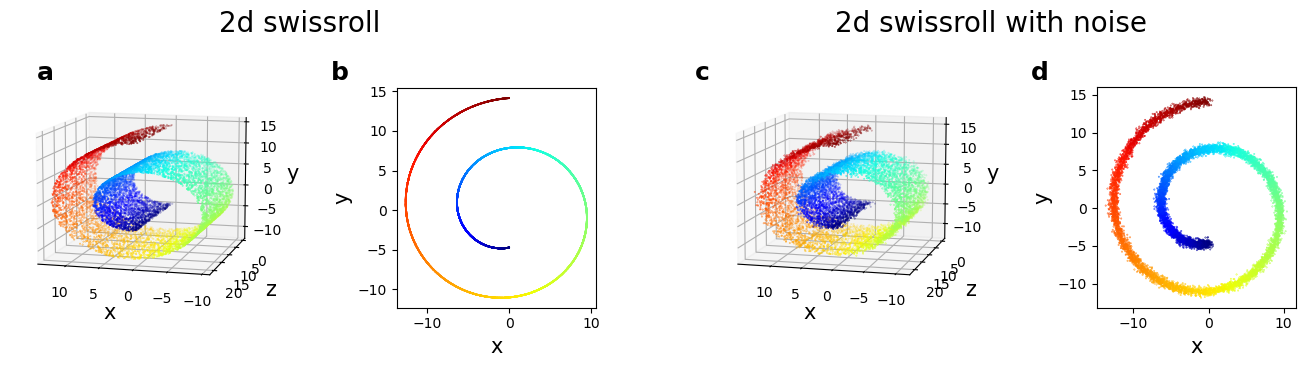
The ID of the noiseless swissroll is comparable to the true ID (\(\sim 2\)). The typical distance :math:`r` is much smaller the the dimension of the manifold (\(\sim 20\), see fig. a)

Adding a gaussian noise to the data with standard deviation \(\sigma=0.3\) (see fig. c, d) the ID increases to reach almost 3.

In this case, the typical distance :math:`r_{noisy}` between the first two neighbors is of the same order of \(\sigma\). The twoNN estimator can not distinguish the ‘noise’ direction from the two relevant directions tangent the data manifold (also named soft directions).

To identify the ‘correct’ intrinsic dimension we need to increase the neighborhood range. In the next part of the tutorial we show two solutions to address this challenge.

Analysis of the ID of noisy datasets: twoNN vs gride

Synthetic datasets: noisy plane, noisy spirals

[20]:

import numpy as np
from mpl_toolkits.mplot3d import Axes3D
from sklearn.datasets import make_swiss_roll
import matplotlib.pyplot as plt
import seaborn as sns
from matplotlib.gridspec import GridSpec


# 2d plane with noise embedded in 3d
ndata = 5000
noise_plane = 0.01
X = np.random.normal(size=(ndata, 2))
X_plane = np.random.normal(scale=noise_plane, size=(ndata, 3))
X_plane[:, :2] = X

# 1d spiral with noise embedded in 3d
ndata = 5000
noise1 = 0.05
t = np.random.uniform(0, 10, ndata)
spiral1 = np.array([t * np.cos(t), t * np.sin(t), t]).T + noise1 * np.random.rand(
    ndata, 3
)

# 2d spiral with noise embedded in 3d
n_samples = 10000
noise2 = 0.3
spiral2, t = make_swiss_roll(n_samples, noise=noise2)
# *******************************************************************************************************

# plot
fig = plt.figure(figsize=(14, 4))
gs = GridSpec(1, 1)

ax = fig.add_subplot(gs[0], projection="3d")
ax.scatter(X_plane[:, 0], X_plane[:, 1], X_plane[:, 2], s=0.1)
ax.set_zlim(-0.2, 0.2)
ax.set_title("noisy plane", fontsize=15)
ax.view_init(10, 105)
gs.tight_layout(fig, rect=[0.1, 0.0, 0.35, 1])


gs = GridSpec(1, 1)
ax = fig.add_subplot(gs[0], projection="3d")
ax.scatter(spiral1[:, 0], spiral1[:, 1], spiral1[:, 2], s=0.1)
ax.set_title("noisy 1d spiral", fontsize=15)
gs.tight_layout(fig, rect=[0.4, 0.0, 0.65, 1])

gs = GridSpec(1, 1)
ax = fig.add_subplot(gs[0], projection="3d")
ax.scatter(spiral2[:, 0], spiral2[:, 1], spiral2[:, 2], s=0.1, c=t, cmap="jet")
ax.set_title("noisy 2d spiral", fontsize=15)
ax.view_init(10, 105)
gs.tight_layout(fig, rect=[0.7, 0.0, 0.95, 1.0])

fig.text(0.1, 0.78, "a", fontsize=18, weight="bold")
fig.text(0.4, 0.78, "b", fontsize=18, weight="bold")
fig.text(0.7, 0.78, "c", fontsize=18, weight="bold")

/var/folders/c2/kglcjml916z_xncfbyv74pn80000gn/T/ipykernel_4109/1685459742.py:44: UserWarning: This figure includes Axes that are not compatible with tight_layout, so results might be incorrect.
  gs.tight_layout(fig, rect = [0.4, 0., 0.65, 1])
/var/folders/c2/kglcjml916z_xncfbyv74pn80000gn/T/ipykernel_4109/1685459742.py:51: UserWarning: This figure includes Axes that are not compatible with tight_layout, so results might be incorrect.
  gs.tight_layout(fig, rect = [0.7, 0.0, 0.95, 1.])

[20]:

Text(0.7, 0.78, 'c')

Id computation

[21]:

from dadapy import data


def compute_ids_scaling(X, range_max=2048, n_min=20):
    "instantiate data class"
    _data = data.Data(coordinates=X, maxk=100)
    "compute ids scaling gride"
    ids_gride, ids_err_gride, rs_gride = _data.return_id_scaling_gride(
        range_max=range_max
    )
    "compute ids with twoNN + decimation"
    ids_twoNN, ids_err_twoNN, rs_twoNN = _data.return_id_scaling_2NN(n_min=n_min)
    return ids_gride, ids_twoNN, rs_gride, rs_twoNN


# *************************************************************

ids_plane_gride, ids_plane_twoNN, rs_plane_gride, rs_plane_twoNN = compute_ids_scaling(
    X_plane, range_max=X_plane.shape[0] - 1, n_min=20
)

(
    ids_spiral1_gride,
    ids_spiral1_twoNN,
    rs_spiral1_gride,
    rs_spiral1_twoNN,
) = compute_ids_scaling(spiral1, range_max=spiral1.shape[0] - 1, n_min=20)

(
    ids_spiral2_gride,
    ids_spiral2_twoNN,
    rs_spiral2_gride,
    rs_spiral2_twoNN,
) = compute_ids_scaling(spiral2, range_max=(spiral2.shape[0] - 1) // 4, n_min=20)

Results and comments

[22]:

import matplotlib.pyplot as plt
import seaborn as sns
from matplotlib.gridspec import GridSpec

fig = plt.figure(figsize=(16, 3))
gs = GridSpec(1, 5)

ax = fig.add_subplot(gs[0])
xrange = min(len(ids_plane_gride), len(ids_plane_twoNN))
sns.lineplot(ax=ax, x=rs_plane_gride, y=ids_plane_gride, label="Gride", marker="o")
sns.lineplot(ax=ax, x=rs_plane_twoNN, y=ids_plane_twoNN, label="twoNN", marker="o")
ax.set_xscale("log")
ax.set_title("noisy plane", fontsize=15)
ax.set_ylabel("ID", fontsize=14)
ax.set_xlabel("distance range", fontsize=14)
ax.axhline(2, color="black", alpha=1, label="true ID", linewidth=0.8)
# ax.axvline(noise_plane, color = 'black', alpha = 1, label = 'noise scale', linewidth = 0.8, linestyle= 'dotted')
ax.legend(fontsize=10)

ax = fig.add_subplot(gs[1])
xrange = min(len(ids_spiral1_gride), len(ids_spiral1_twoNN))
sns.lineplot(ax=ax, x=rs_spiral1_gride, y=ids_spiral1_gride, label="Gride", marker="o")
sns.lineplot(ax=ax, x=rs_spiral1_twoNN, y=ids_spiral1_twoNN, label="twoNN", marker="o")
ax.set_xscale("log")
ax.set_title("1d noisy spiral", fontsize=15)
ax.set_xlabel("distance range", fontsize=14)
ax.axhline(1, color="black", alpha=1, label="true ID", linewidth=0.8)
ax.axvline(
    noise1, color="black", alpha=1, label="noise std", linewidth=0.8, linestyle="dashed"
)
ax.legend(fontsize=10)
gs.tight_layout(fig)


ax = fig.add_subplot(gs[2])
xrange = min(len(ids_spiral2_gride), len(ids_spiral2_twoNN))
sns.lineplot(ax=ax, x=rs_spiral2_gride, y=ids_spiral2_gride, label="Gride", marker="o")
sns.lineplot(ax=ax, x=rs_spiral2_twoNN, y=ids_spiral2_twoNN, label="twoNN", marker="o")
ax.set_xscale("log")
ax.set_title("2d noisy spiral", fontsize=15)
ax.set_xlabel("distance range", fontsize=14)
ax.axhline(2, color="black", alpha=1, label="true ID", linewidth=0.8)
ax.axvline(
    noise2, color="black", alpha=1, label="noise std", linewidth=0.8, linestyle="dashed"
)
ax.legend(fontsize=10)
gs.tight_layout(fig)


ax = fig.add_subplot(gs[3])
xrange = min(len(ids_spiral2_gride), len(ids_spiral2_twoNN))
x = spiral2.shape[0] / np.array([2**i for i in range(xrange)])
sns.lineplot(ax=ax, x=x, y=ids_spiral2_gride[:xrange], label="Gride", marker="o")
sns.lineplot(ax=ax, x=x, y=ids_spiral2_twoNN[:xrange], label="twoNN", marker="o")
ax.legend(fontsize=10)
ax.set_xscale("log")
ax.set_title("2d noisy spiral", fontsize=15)
ax.set_xlabel("n° data", fontsize=14)
# ax.set_xticks(x, x[::-1])
ax.axhline(2, color="black", alpha=1, label="true ID", linewidth=0.8)
ax.legend(fontsize=10)


fig.text(0.04, 0.9, "a", fontsize=18, weight="bold")
fig.text(0.24, 0.9, "b", fontsize=18, weight="bold")
fig.text(0.43, 0.9, "c", fontsize=18, weight="bold")
fig.text(0.63, 0.9, "d", fontsize=18, weight="bold")

[22]:

Text(0.63, 0.9, 'd')

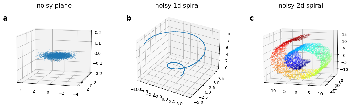
The variance of the noise directions are is much smaller than size of the manifold. For example, in our syntetic datasets (fig. a, b, c-d) the noise standard deviation is few percents of size of the dataset.

When the typical distance involved in the ID estimate becomes larger than the noise scale (but sufficilently smaller than the size of the dataset) the intrinsic dimension approaces a value consistent with the number of soft directions of the data. If the noise variance is much smaller from than the variance of the data, the ID as a function of the typical distance exhibits a plateau.

To identify the ID we look for plateaus in the plot the ID vs scale.

Strategies to increase the scale

TwoNN: increases the typical distance by bootstrapping random subsets of data, and measures the ID on such subsets with progressively fewer datapoints. The typical distance for a random subset of \(N^*\) points is:

r = \(\frac{1}{N_{dec}} \sum \limits_{i=1}^{N_{dec}} \frac{r_{1i}+r_{2i}}{2}\)

this is what is plotted on the x axis for the TwoNN estimator (Fig. a, b, c ).

Gride: increases the typical distance by considering neighbors of higher order and measures the ID on the full dataset. The typical distance considering neighbors of order n and 2n is:

\(r_n = \frac{1}{N} \sum \limits_{i=1}^{N} \frac{r_{n_i}+r_{2n_i}}{2}\)

the average is taken over all the N datapoints. This is what is plotted on the x axis for the Gride estimator (Fig. a, b, c ).

Scale analysis when the intrinsic dimension is high

When the ID is high (say, ID>5-10) the concentration of measure makes all the distances comparable. To analyze how the ID varies with the scale we plot (see Fig. d):

Rule 1

IDs vs N/n1for theGrideestimator;
IDs vs N_decfor thetwoNNestimator

where:

n1: order of the first neighbors involved in the gride estimate. They are n1 = [1, 2, 4, 8, …, log2(range_scaling)] and \(n2 = 2 \cdot n1\)
N_dec (twoNN): size of the decimated dataset. It is N/[1, 2, 4, 8, …] up to N_min

We typically plot the x axis in logarithmic scale.

The constant factor N in N/n1 (Gride estimator), makes the x-axis easy to compare with the twoNN estimator. Indeed, the average distances used by Gride for n1=2 (n2=4) is comparable to that of the twoNN estimator evaluated on half of the datapoints see Fig. d.

We also notice that when the ID is small rule1 is equivalent to the more intuitive plot IDs vs average distance (compare Figs. c and d).

Real datastes: mnist, isomap faces, isolet voices

[23]:

from urllib.request import urlretrieve
from collections import namedtuple
from os.path import exists
import matplotlib.pyplot as plt
import numpy as np


def fetch_data(data_path, data_url, force_download=True):
    if not exists(data_path) or force_download:
        print(f"downloading data from {data_url} to {data_path}")
        urlretrieve(data_url, data_path)
        dataset = np.load(data_path)
    else:
        dataset = np.load(data_path)
    return dataset


# mnist and isolet datasets
RemoteFileMetadata = namedtuple("RemoteFileMetadata", ["filename", "url"])
isolet = RemoteFileMetadata(
    filename="isolet_float32.npy", url="https://figshare.com/ndownloader/files/34882686"
)
mnist = RemoteFileMetadata(
    filename="mnist.npy", url="https://figshare.com/ndownloader/files/34882689"
)
faces = RemoteFileMetadata(
    filename="isomap_faces.npy", url="https://figshare.com/ndownloader/files/34894287"
)

faces_data = fetch_data(f"./datasets/{faces.filename}", faces.url, force_download=False)
print(f"isomap_faces shape: N data x P features = {faces_data.shape}")

isolet_data = fetch_data(
    f"./datasets/{isolet.filename}", isolet.url, force_download=False
)
print(f"isolet shape: N data x P features = {isolet_data.shape}")

mnist_data = fetch_data(f"./datasets/{mnist.filename}", mnist.url, force_download=False)
mnist_data = mnist_data.astype("float")
print(f"mnist 1 digit shape: N data x P features = {mnist_data.shape}")

# ************************************************************************************************
# plot
fig = plt.figure(figsize=(8, 3))
gs = GridSpec(1, 3)

ax = fig.add_subplot(gs[1])
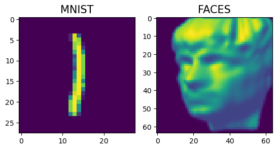
ax.imshow(mnist_data[10].reshape(28, 28))
ax.set_title("MNIST", fontsize=15)

ax = fig.add_subplot(gs[2])
ax.imshow(faces_data[0].reshape(64, 64).T)
ax.set_title("FACES", fontsize=15)

gs.tight_layout(fig)

isomap_faces shape: N data x P features = (698, 4096)
isolet shape: N data x P features = (7797, 617)
mnist 1 digit shape: N data x P features = (6742, 784)

ID computation

This may take up to 20/30 seconds

[24]:

from dadapy import data


def compute_ids_scaling(X, range_max=2048, n_min=20):
    "instantiate data class"
    _data = data.Data(coordinates=X, maxk=100)
    "compute ids scaling gride"
    ids_gride, ids_err_gride, rs_gride = _data.return_id_scaling_gride(
        range_max=range_max
    )
    "compute ids with twoNN + decimation"
    ids_twoNN, ids_err_twoNN, rs_twoNN = _data.return_id_scaling_2NN(n_min=n_min)
    return ids_gride, ids_twoNN, rs_gride, rs_twoNN


"this may take from 10 to 20 seconds"
ids_mnist_gride, ids_mnist_twoNN, _, _ = compute_ids_scaling(
    mnist_data, range_max=2048, n_min=20
)
ids_faces_gride, ids_faces_twoNN, _, _ = compute_ids_scaling(
    faces_data, range_max=2048, n_min=20
)
ids_isolet_gride, ids_isolet_twoNN, _, _ = compute_ids_scaling(
    isolet_data, range_max=2048, n_min=20
)

Results and comments

[25]:

import matplotlib.pyplot as plt
import seaborn as sns
from matplotlib.gridspec import GridSpec

fig = plt.figure(figsize=(10, 3))
gs = GridSpec(1, 3)

ax = fig.add_subplot(gs[0])
xrange = min(len(ids_mnist_gride), len(ids_mnist_twoNN))
x = mnist_data.shape[0] / np.array([2**i for i in range(xrange)])
sns.lineplot(ax=ax, x=x, y=ids_mnist_gride[:xrange], label="Gride", marker="o")
sns.lineplot(ax=ax, x=x, y=ids_mnist_twoNN[:xrange], label="twoNN", marker="o")
ax.legend(fontsize=10)
ax.set_xscale("log")
ax.set_title("MNIST digit 1", fontsize=15)
# ax.set_ylabel('ID', fontsize = 14)
ax.set_xlabel("n° data", fontsize=14)
ax.axhspan(8, 11, color="C2", alpha=0.1)

ax = fig.add_subplot(gs[1])
xrange = min(len(ids_faces_gride), len(ids_faces_twoNN))
x = mnist_data.shape[0] / np.array([2**i for i in range(xrange)])
sns.lineplot(ax=ax, x=x, y=ids_faces_gride[:xrange], label="Gride", marker="o")
sns.lineplot(ax=ax, x=x, y=ids_faces_twoNN[:xrange], label="twoNN", marker="o")
ax.set_xscale("log")
ax.set_title("FACES", fontsize=15)
# ax.set_ylabel('ID', fontsize = 14)
ax.set_xlabel("n° data", fontsize=14)
ax.axhline(3, color="black", label="true ID", linewidth=0.8)
ax.legend(fontsize=10)


ax = fig.add_subplot(gs[2])
xrange = min(len(ids_isolet_gride), len(ids_isolet_twoNN))
x = isolet_data.shape[0] / np.array([2**i for i in range(xrange)])
sns.lineplot(ax=ax, x=x, y=ids_isolet_gride[:xrange], label="Gride", marker="o")
sns.lineplot(ax=ax, x=x, y=ids_isolet_twoNN[:xrange], label="twoNN", marker="o")
ax.legend(fontsize=10)
ax.set_xscale("log")
ax.set_title("Isolet", fontsize=15)
# ax.set_ylabel('ID', fontsize = 14)
ax.set_xlabel("n° data", fontsize=14)
ax.axhspan(16, 22, color="C2", alpha=0.1)

gs.tight_layout(fig)

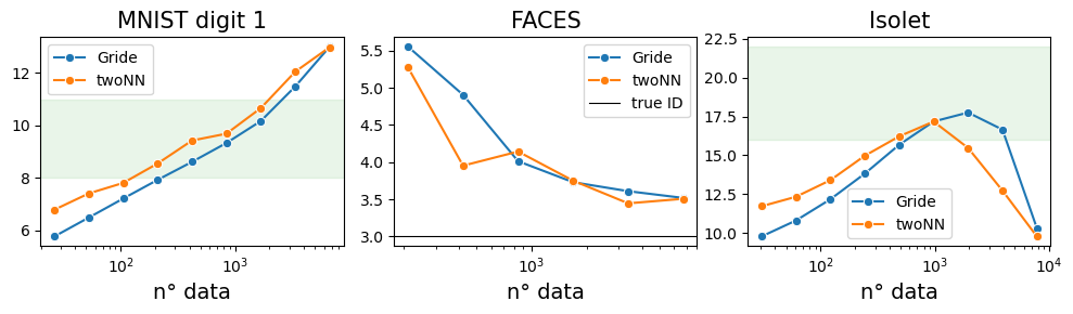
When the ID is high the concentration of measure makes all the distances comparable and rule1 becomes the only sensible way to go. The ground truth ID for these datasets is not known, but there is a (debatable) consensus for the plausible range of IDs of each of them. This range is highlighted in the figures. The plateau for the MNIST dataset Fig. c is absent, for the face dataset is around 3.5/3.6, for the isolet dataset is around 17.5 for Gride, 16 for twoNN.

When the plateau is absent we typically choose as ID the Gride estimate with (n1=2, n2=4), or (n1=4, n2=8), or an average of these.